[Explainable AI] LIME 으로 머신러닝 모델을 해석해보자

2022-01-12 6 분 소요

Explainable AI(설명 가능한 인공지능)의 대표적인 기법인 LIME을 tabular data 에 적용하여 모델을 해석해보자.

Project Setup
Data Cleansing
Data Modelling
Model Validation
Explainability with LIME

Project Setup

try:
  import lime
except:
  !pip install lime
  import lime

# Importing necessary libraries
import pandas as pd

from sklearn.preprocessing import OneHotEncoder, StandardScaler
from sklearn.impute import SimpleImputer
from sklearn.ensemble import RandomForestClassifier
from sklearn.model_selection import train_test_split, GridSearchCV
from sklearn.metrics import roc_auc_score, accuracy_score, confusion_matrix

import lime.lime_tabular

import warnings
warnings.filterwarnings('ignore')

# Importing the training data
df_train = pd.read_csv('/content/train.csv')

# Viewing the first few rows of the data
df_train.head()

	PassengerId	Survived	Pclass	Name	Sex	Age	SibSp	Ticket	Fare	Cabin	Embarked
0	1	0	3	Braund, Mr. Owen Harris	male	22.0	1	A/5 21171	7.2500	NaN	S
1	2	1	1	Cumings, Mrs. John Bradley (Florence Briggs Th...	female	38.0	1	PC 17599	71.2833	C85	C
2	3	1	3	Heikkinen, Miss. Laina	female	26.0	0	STON/O2. 3101282	7.9250	NaN	S
3	4	1	1	Futrelle, Mrs. Jacques Heath (Lily May Peel)	female	35.0	1	113803	53.1000	C123	S
4	5	0	3	Allen, Mr. William Henry	male	35.0	0	373450	8.0500	NaN	S

Return to top of notebook

Data Cleansing & Feature Engineering

Age -> Age Bins: child, teen, young adult, adult, elder, or unknown
Cabin -> Section: A, B, C, or no cabin

불필요한 칼럼 Drop

df_train.drop(columns = ['PassengerId', 'Name', 'Ticket'], inplace = True)

“Age” 칼럼 정보에서 “age_bins” feature 만들어 Age칼럼 대체

# Defining / instantiating the necessary variables
age_bins = [-3, -1, 12, 18, 25, 50, 100]
age_labels = ['unknown', 'child', 'teen', 'young_adult', 'adult', 'elder']
# Filling null age values
df_train['Age'] = df_train['Age'].fillna(-2)
# Binning the ages appropriate as defined via the variables above
df_train['Age_Bins'] = pd.cut(df_train['Age'], bins = age_bins, labels = age_labels)
# Dropping the now unneeded 'Age' feature
df_train.drop(columns = 'Age', inplace = True)

“Cabin” 칼럼 정보에서 맨 앞 한글자씩 따서 “Section” feature 만들어 Cabin 대체

C85 becomes “C”

# Grabbing the first character from the cabin section
df_train['Section'] = df_train['Cabin'].str[:1]
# Filling out the nulls
df_train['Section'].fillna('No Cabin', inplace = True)
# Dropping former 'Cabin' feature
df_train.drop(columns = 'Cabin', inplace = True)

“Embarked” 칼럼: 결측치 Unknown 으로 채우기

df_train['Embarked'] = df_train['Embarked'].fillna('Unknown')

Categorical variables 에 대해 One hot encoding

# Defining the categorical features
cat_feats = ['Pclass', 'Sex', 'Age_Bins', 'Embarked', 'Section']
# Instantiating OneHotEncoder
ohe = OneHotEncoder(categories = 'auto')
# Fitting the categorical variables to the encoder
cat_feats_encoded = ohe.fit_transform(df_train[cat_feats])
# Creating a DataFrame with the encoded value information
cat_df = pd.DataFrame(data = cat_feats_encoded.toarray(), columns = ohe.get_feature_names(cat_feats))

Numerical columns에 대해 Scaling

# Defining the numerical features
num_feats = ['SibSp', 'Parch', 'Fare']
# Instantiating the StandardScaler object
scaler = StandardScaler()
# Fitting the data to the scaler
num_feats_scaled = scaler.fit_transform(df_train[num_feats])
# Creating DataFrame with numerically scaled data
num_df = pd.DataFrame(data = num_feats_scaled, columns = num_feats)

Encoded & Scaled 된 Dataframes 들을 Concatenate 해서 “X” 라는 training data 만들기

X = pd.concat([cat_df, num_df], axis = 1)

df_train 에서 target 변수 (“Survived”) 를 “y”로 지정

y = df_train[['Survived']]

Training / Validation Split

X_train, X_val, y_train, y_val = train_test_split(X, y, random_state = 42)

Return to top of notebook

Data Modelling

GridSearch 로 optimal 파라미터 찾기

# Defining the random forest parameters
params = {'n_estimators': [10, 50, 100],
          'min_samples_split': [2, 5, 10],
          'min_samples_leaf': [1, 2, 5],
          'max_depth': [10, 20, 50]
         }
         
# Instantiating RandomForestClassifier object and GridSearch object
rfc = RandomForestClassifier()
clf = GridSearchCV(estimator = rfc,
                   param_grid = params)
# Fitting the training data to the GridSearch object
clf.fit(X_train, y_train)

GridSearchCV(estimator=RandomForestClassifier(),
             param_grid={'max_depth': [10, 20, 50],
                         'min_samples_leaf': [1, 2, 5],
                         'min_samples_split': [2, 5, 10],
                         'n_estimators': [10, 50, 100]})

# Displaying the best parameters from the GridSearch object
clf.best_params_

{'max_depth': 50,
 'min_samples_leaf': 2,
 'min_samples_split': 5,
 'n_estimators': 50}

Training the model with the ideal params

# Instantiating RandomForestClassifier with ideal params
rfc = RandomForestClassifier(max_depth = 10,
                             min_samples_leaf = 2,
                             min_samples_split = 2,
                             n_estimators = 10)

# Fitting the training data to the model
rfc.fit(X_train, y_train)

RandomForestClassifier(max_depth=10, min_samples_leaf=2, n_estimators=10)

Return to top of notebook

LIME 해석 위한 예시 데이터

Validation set 에서 Survived 와 did not survive 각각 준비

# Contentating X_val and y_val into single df_val set
df_val = pd.concat([X_val, y_val], axis = 1)

# Viewing first few rows of df_val to hopefully find 2 good candidates for our study
df_val.head()

	Pclass_2	Pclass_3	Sex_female	Sex_male	Age_Bins_adult	Age_Bins_child	Age_Bins_teen	Age_Bins_unknown	Age_Bins_young_adult	Embarked_C	Embarked_S	Section_No Cabin	SibSp	Parch	Fare	Survived
709	0.0	1.0	0.0	1.0	0.0	0.0	0.0	1.0	0.0	1.0	0.0	1.0	0.432793	0.767630	-0.341452	1
439	1.0	0.0	0.0	1.0	1.0	0.0	0.0	0.0	0.0	0.0	1.0	1.0	-0.474545	-0.473674	-0.437007	0
840	0.0	1.0	0.0	1.0	0.0	0.0	0.0	0.0	1.0	0.0	1.0	1.0	-0.474545	-0.473674	-0.488854	0
720	1.0	0.0	1.0	0.0	0.0	1.0	0.0	0.0	0.0	0.0	1.0	1.0	-0.474545	0.767630	0.016023	1
39	0.0	1.0	1.0	0.0	0.0	0.0	1.0	0.0	0.0	1.0	0.0	1.0	0.432793	-0.473674	-0.422074	1

# Noting the two respective people
person_1 = X_val.loc[[720]] # Survived
person_2 = X_val.loc[[439]] # Did not Survive

Explainability with LIME

Instantiate LIME tabular

Tabular Data 에 대해서 LIME represents a weighted combination of columns
Args/Parameters
- 1) training_data: numpy 2d array
- 2) mode: “classification” or “regression”
- 3) feature_names: list of names (strings) corresponding to the columns in the training data
- 4) class_names: list of class names, ordered according to whatever the classifier is using. If not present, class names will be ‘0’, ‘1’, …

# Importing LIME
import lime.lime_tabular

# Defining our LIME explainer
lime_explainer = lime.lime_tabular.LimeTabularExplainer(X_train.values,
                                                        mode = 'classification',
                                                        feature_names = X_train.columns,
                                                        class_names = ['Did Not Survive', 'Survived']
                                                        )

# Defining a quick function that can be used to explain the instance passed
predict_rfc_prob = lambda x: rfc.predict_proba(x).astype(float)

두 가지 케이스에 대한 LIME 해석

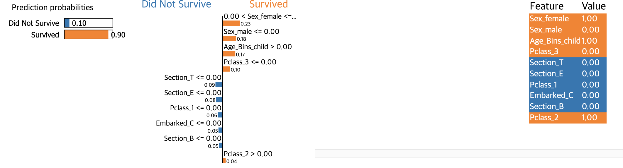
케이스 1)

왼쪽 패널 ▶ Random Forest Model 은 “Survived” 일 거라고 거의 100% 예측했다
중앙 패널 ▶ 특정 데이터 포인트의 각각의 feature 를 통해 (중요도순) 예측을 설명하고자 한다
- 이 사람(sample)의 Sex_female feature에 대한 value는 1인데, 0<Sex_female<=1 에 해당되므로 “Survived” 라고 분류될 경향이 더 높다
- 같은 원리로 이 샘플 Sex_male <= 0 에 해당하기 때문에, “Survived” 라고 분류될 경향이 더 높다
- 이 샘플은 Age_Bins_child = 1 이므로, Age_Bins_child > 0.00 에 해당하기 때문에 “Survived” 라고 분류될 경향이 더 높다
- 그런가하면 Section_E 는 다른 해석을 내놓았다. Section_E= 0 이므로, Section_E <= 0.00 에 해당하기 때문에 “Did Not Survive” 라고 설명한다
오른쪽 패널 ▶ 이 샘플의 features & values 를 나타낸다

person_1_lime = lime_explainer.explain_instance(person_1.iloc[0].values,
                                                predict_rfc_prob,
                                                num_features = 10)
person_1_lime.show_in_notebook()
# person_1_lime.save_to_file("person_1.html")

lime_case1

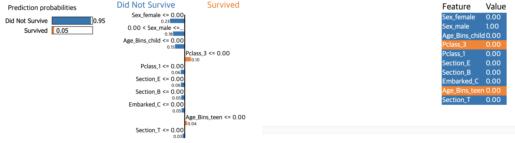
케이스 2)

왼쪽 패널 ▶ Random Forest Model 은 아래 샘플이 “Did Not Survive” 일 거라고 94% 예측했다
중앙 패널 ▶ 특정 데이터 포인트의 각각의 feature 를 통해 (중요도순) 예측을 설명하고자 한다
- 이 사람(sample)의 Sex_female feature에 대한 value는 1인데, 0<Sex_female<=1 에 해당되므로 “Did Not Survive” 라고 예측한 것에 대한 설명력이 높다
- 같은 원리로 이 샘플 Sex_male <= 0 에 해당하기 때문에, “Did Not Survive” 라고 분류될 경향이 더 높다
- 이 샘플은 Age_Bins_child = 0 이므로, Age_Bins_child <= 0.00 에 해당하기 때문에 “Did Not Survive” 라고 분류될 경향이 더 높다
- 또한, 이 샘플은 Section_E = 0 이므로, Section_E <= 0.00 에 해당하기 때문에 “Did Not Survive” 라고 분류될 경향이 더 높다
- 그런가하면 Pclass_3 는 다른 해석을 내놓았다. Pclass_3= 0 이므로, Pclass_3 <= 0.00 에 해당하기 때문에 “Survived” 라고 설명한다
오른쪽 패널 ▶ 이 샘플의 features & values 를 나타낸다

person_2_lime = lime_explainer.explain_instance(person_2.iloc[0].values,
                                                predict_rfc_prob,
                                                num_features = 10)
person_2_lime.show_in_notebook()
# person_2_lime.save_to_file("person_2.html")

lime_case2

Return to top of notebook

To Do & consideration

Categorical / Numerical 변수들이 많을 때 얼마나 많은 데이터를 갖고 설명해야할지에 대한 선?

Reference

Twitter Facebook LinkedIn

[Explainable AI] LIME 으로 머신러닝 모델을 해석해보자

Table of Contents

Project Setup

Data Cleansing & Feature Engineering

불필요한 칼럼 Drop

“Age” 칼럼 정보에서 “age_bins” feature 만들어 Age칼럼 대체

“Cabin” 칼럼 정보에서 맨 앞 한글자씩 따서 “Section” feature 만들어 Cabin 대체

“Embarked” 칼럼: 결측치 Unknown 으로 채우기

Categorical variables 에 대해 One hot encoding

Numerical columns에 대해 Scaling

Encoded & Scaled 된 Dataframes 들을 Concatenate 해서 “X” 라는 training data 만들기

df_train 에서 target 변수 (“Survived”) 를 “y”로 지정

Training / Validation Split

Data Modelling

GridSearch 로 optimal 파라미터 찾기

Training the model with the ideal params

LIME 해석 위한 예시 데이터

Validation set 에서 Survived 와 did not survive 각각 준비

Explainability with LIME

Instantiate LIME tabular

두 가지 케이스에 대한 LIME 해석

케이스 1)

케이스 2)

To Do & consideration

Reference

공유하기

댓글남기기

참고

[OCR/AI] 네이버 클로바(Clova) OCR 모델 API 신청부터 직접 사용해보기(feat.코랩)

[에러 해결] Python urlopen error [SSL: CERTIFICATE_VERIFY_FAILED]

[AI 소식] 제미나이(Gemini)란? GPT-4보다 뛰어난 구글의 AI 모델 소개 및 간단 사용 후기 & 논란

[OCR/AI] Upstage OCR 모델 API 신청부터 직접 사용해보자(코랩)